Master the Checkmark: A Complete Guide for Google Sheets

Checkmarks (✓) are a versatile way to track progress, create to-do lists, or visually mark completed tasks within your Google Sheets spreadsheets. Whether you’re a beginner or a seasoned Sheets user, this guide will explore various methods to add checkmarks and even customize them to your preferences.

Why Use Checkmarks in Google Sheets?

• Visual Clarity: Checkmarks offer a quick visual cue to see what’s done and what’s pending.
• Organization: They can transform your sheet into an interactive checklist.
• Data Validation: Checkboxes (which display as checkmarks) can be linked to custom values, enhancing data analysis and automation.

Method 1: Inserting Interactive Checkboxes

This is the most straightforward and functional approach:

1. Select Cells: Highlight the cells where you want checkboxes to appear.
2. Insert Checkbox:
   • Go to the menu bar and click “Insert.”
   • Select “Checkbox.”
3. Click to Check/Uncheck: Clicking the box toggles the checkmark on or off.

Key Tip: You can easily copy and paste a single checkbox to fill other cells.

Method 2: Typing the Checkmark Character

If you need a simple checkmark symbol without the interactivity of a checkbox:

1. Select Cell: Choose the cell where you want the checkmark.
2. Keyboard Shortcut:
   • On Windows: Hold down the Alt key and type 0252 on the numeric keypad.
   • On Mac: Hold down Option and type V.
3. Alternative: Copy and paste the checkmark symbol (✓) from this guide or another source.

Method 3: Using the CHAR Function

For those comfortable with formulas, the CHAR function provides another option:

1. Enter Formula: In the desired cell, type =CHAR(10003)
2. Press Enter: The checkmark symbol will appear.

Advanced Tip: Use conditional formatting to automatically apply checkmarks based on cell values (e.g., “Yes” or “Complete”).

Related: Why does my Google Chrome keep quitting unexpectedly on Mac?

Method 4: Custom Checkboxes with Data Validation

Image Source

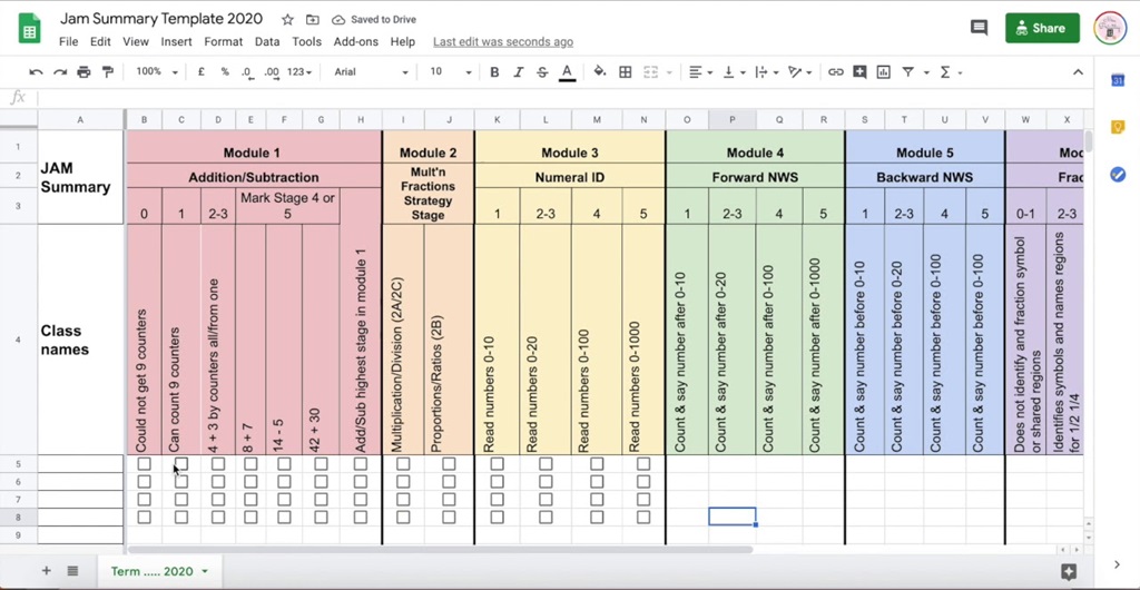
This method is ideal for linking checkmarks to specific values (e.g., “Yes/No” or “True/False”):

1. Select Cells: Choose the range where you want the checkboxes.
2. Data Validation:
   • Go to “Data” in the menu and select “Data validation.”
   • In the “Criteria” dropdown, select “Checkbox.”
   • Under “Use custom cell values,” enter your desired checked/unchecked values (e.g., “Yes” for checked, “No” for unchecked).
   • Click “Save.”

Method 5: Special Characters and Emoji

For a bit of fun, you can use alternative checkmark symbols:

1. Insert Menu: Go to “Insert” > “Special characters.”
2. Search: Type “checkmark” or “check” to find different symbols.
3. Emoji: Use your computer’s emoji keyboard (usually accessible with a keyboard shortcut).

Customization Tips

• Colors: Change the color of checkboxes using conditional formatting.
• Symbols: Use the CHAR function with different codes to find alternative symbols.
• Checkbox Size: Adjust cell height and width to resize the checkbox.

Troubleshooting

• Checkmark Not Appearing: If you’re using the keyboard shortcut, ensure Num Lock is enabled.
• Function Errors: Double-check your formulas for typos.

Beyond Checkmarks

Google Sheets offers a variety of other tools to visually enhance and organize your data, including:

• Conditional Formatting: Change colors, add icons, or even create progress bars based on cell values.
• Data Validation Dropdowns: Create interactive lists with pre-defined options.
• Sparkline Charts: Insert mini-charts directly into cells to visualize trends.

Let me know if you’d like a deeper dive into any of these methods or have other Google Sheets questions!

Featured Image Source